Decrease Battery Testing Time Using Multisine EIS

Introduction

Gamry Instrument’s multisine Electrochemical Impedance Spectroscopy (EIS) has the potential to decrease battery testing time by over a factor of three. EIS has become a standard technique in the testing of batteries and battery materials. This non-destructive technique allows the examination of multiple characteristics with the battery itself within a single experiment.

Researchers are able to examine processes taking place at the anode, cathode, separator, or even within the electrolyte itself.

This is because an alternative current (or voltage) sinewave is applied to the battery at a range of frequencies. The battery’s response is then measured at each of these frequencies and this response is converted into an impedance. Examining changes in impedance at different charge states or over the lifetime of a battery gives insights into battery behavior and degradation processes.

EIS is typically done by applying one frequency at a time and measuring the battery’s response. Then the next frequency is applied the process is repeated. If EIS suffers from one setback it is that at lower frequencies, the process can take up to an hour or more to complete.

There is an alternative however that can reduce testing time by over a factor of three. By applying multiple sine waves to the battery and measuring the cells response, the researcher can get the same information in less time. Compounding this time savings over multiple cells over a long timeframe can save significant time and resources for the researcher.

However, this time savings comes at the expense of more noise within the measurement. Gamry Instrument’s compensates for this increase in noise several ways. This article is going to quickly walk you through how single sine EIS is done followed by how Gamry Instruments has implemented multisine EIS.

How is EIS Done?

Single-Sine EIS measurements involve applying a sinusoidal perturbation (voltage or current) and measuring the response (current or voltage respectively). The measurement is complete when it is deemed to be satisfactory, or some time limit is reached.

This decision requires a mathematically sound criterion for a satisfactory measurement. Gamry Instrument’s Single-Sine technique terminates the measurement at each frequency when its signal to noise ratio exceeds a target value.

Power in the measured signal can be written, using Parseval’s Theorem, as the sum of three components, DC, AC and noise. Algebraically this is:

  

(1)

where, x_n, is the time series of the measured signal, ₀ is the DC component, ₁ is the AC component of interest and  are the noise and distortion components in the unexcited harmonics. Pictorially, Equation 1 can be depicted as the decomposition of a noisy sine wave as shown in Figure 1.

Figure 1. The partition of a noisy sine wave. Three components are shown on the right. DC (top), AC (middle), Noise (bottom).

The AC and DC components can be easily calculated in real time as points in xn become available using:

The noise power is calculated by subtracting the AC power and DC power from the total power. The signal to noise ratio (SNR) is defined as the ratio of power in the desired AC component to the noise power. SNR is monitored throughout the measurement and the measurement is deemed complete when its value goes above a predefined value.

This procedure is repeated for every frequency of interest, generating the full spectrum.
Because the noise component is random; averaging the measurement decreases the noise power thereby increasing the signal to noise ratio. To avoid infinite loops when systematic noise does not average out, we also limit the maximum cycles at any frequency.

The time it takes to acquire the spectrum depends heavily on the frequencies of interest and the signal to noise characteristics of the attempted measurement. A typical lower frequency limit is 1 mHz, where each single sine wave cycle takes 1000 sec.

Furthermore, starting from a zero potential or a zero current condition, any battery takes some time to settle to a steady state response to an applied sine wave. The time it takes to settle depends on the characteristics of the battery and is hard to determine. This causes the initial cycle to be distorted by a startup transient which is excluded from the final calculation.
Depending on the desired number of frequencies and signal to noise ratio, spectral measurement down to 1 mHz can typically take a couple of hours.

In comes multisine EIS
One attempt to shorten the time involved is to simultaneously apply multiple sine waves. This approach has revolutionized a number of analytical chemistry techniques and so Gamry Instruments has applied the same process to battery measurements.

Signal Generation

Generation of the Frequency Table

EIS experiments typically employ logarithmically spaced frequencies over a number of decades. In a multisine experiment, in order to get accurate frequency transforms, all applied sine waves must fit the time window perfectly. Put another way, all the frequencies used must be integer multiples of some fundamental frequency.

Maximizing the frequency window requires some hard decisions about frequency spacing. If a logarithmically spaced frequency spectrum is desired, a fundamental frequency must be far below the minimum frequency of interest. For example, a 10 point/decade logarithmically spaced spectrum requires a fundamental frequency six times longer than the minimum frequency making the overall experiment time six times longer. If however, one can tolerate linearly spaced frequencies for the lower frequency part of the spectrum, one can use the minimum frequency of interest as the fundamental and achieve shorter times.

Gradient Descent Phase Optimization

Adding up sine waves increases the amplitude of the perturbation. In order to ensure the state of the battery does not change, the overall amplitude needs to be kept low. In the worst-case scenario, the amplitude of the total perturbation is the amplitude of the single perturbation multiplied by the number of frequencies. This is the case when all the sine waves are in phase.
Taking an example with 31 sine waves with unity amplitudes, the worst-case scenario exhibits the pattern shown in Figure 2 . Notice the total amplitude at the midpoint of the pattern is the same as the number of sine waves used.

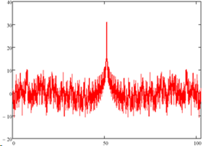
Figure 2. The worst case phase signal vs time. All component phases set to maximum at midpoint.

This worst case scenario is highly undesirable and could possibly damage the battery. Randomizing the phase of the excitation sine waves is a good first step in lowering the excitation amplitude. For the frequencies in Figure 2, one random set of phases results in the pattern in Figure 3. Notice that the peak value decreased from 31 to about 15.  

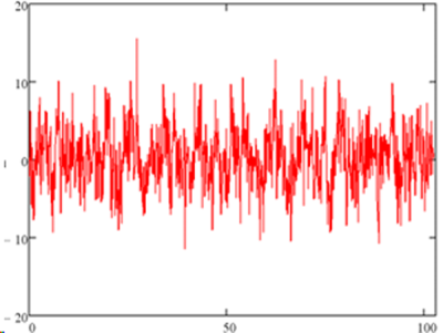
Figure 3. The same signal with randomized phases.

One can try a number of non-linear optimization methods to decrease the likelihood of a worst-case scenario and increase the reproducibility2, .Due to the nature of the problem, there are a number of local minima that are very closely spaced. Any minimization algorithm will have a hard time finding the optimum phase set. We have implemented the method developed by Farden et. al.8. where an algorithm goes through iterations of finding the absolute maximum in a given signal and modifying the phases in order to decrease the amplitude at that given time value. Or, more mathematically, takes a steepest descent step in phase space. The optimized result for our particular example is shown in Figure 4. Notice the maximum amplitude is ~13.

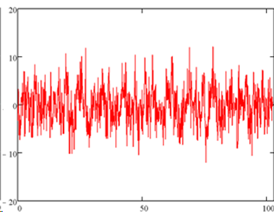
Figure 4. The optimized signal. The same frequencies and amplitudes as Figures 2 and 3 are now optimized using the algorithm explained in the text.

It is possible to tackle the problem from the other side. That is, take a signal definition that is known to have low peak values for given power and try to impose the desired frequency spectrum onto the signal. An example for low peak factor signals is the frequency modulated (FM) signal and it is possible to impose the desired spectrum onto an FM signal. Using this approach, Schroeder reported the closed form expression for the phase shown in Equation 2 below.

         (2)

where  is the phase of the  harmonic and  is the amplitude of the i^th harmonic. For most setsof interest in EIS, the Schroeder signal has a higher peak factor than the result of the phase optimization described above. Anecdotally, the phase set generated by Equation 2 results in a lower peak factor signal than our algorithm if one were to use all existing harmonics between 1 and n. The logarithmically spaced frequencies used in typical EIS experiments, on the other hand, very sparsely fill the integral harmonics and the FM signal does not work as well. 

Calculating Noise

The measurement of signal and noise for the multisine measurement is very similar to the single sine measurement. By extension of Eq. 1 to multiple excitations, one gets:

      (3)

where h_ex are those harmonics that make up the set of desired measurement frequencies and h_un are those frequencies that are not excited. Chosen h_un make up the harmonics that are monitored to get noise estimates for given frequency ranges.

Any given  can be calculated using Equation 4.

      (4)

The definition of a satisfactory measurement is also very similar to the single sine case. We demand that at every frequency of interest, the signal to noise ratio is higher than some predefined value. We now define noise at a frequency to be the power at a nearby unexcited frequency.

Power Leveling

A spectrum measured using uniform amplitudes will show a frequency dependent signal to noise ratio. Both the signal and the noise spectrum will vary with frequency. External interferences or specific characteristics of the electronics used will cause different noise levels at different frequencies. The measured signal will also be different throughout the spectrum. Therefore, averaging the signal in order to achieve the same signal to noise ratio for the entire data set will lead to vastly different times for the measurement to complete.

For example, measuring a 1nF capacitor between 1 Hz and 100 Hz using uniform amplitude signal, leads to the current and voltage spectrum shown in Figure 5.

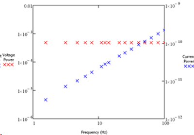
Figure 5. Fourier transforms of a 1nF capacitor measured using unity amplitude potential signal.

Notice the uniform amplitude on the voltage signal that is used as prepared and the current signal being low at the lower frequencies due to the increase in the impedance of the capacitor.
Because the power in the current is not uniform, the signal to noise ratio measured will not be uniform even with a flat noise spectrum. In an attempt to get uniform signal to noise distribution across the spectrum, we can adjust the power on the applied frequencies. The resulting applied voltage and the measured current spectra are shown in Figure 6 .

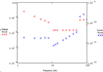
Figure 6. The adjusted applied voltage spectrum and the resulting current spectrum.

Using a power optimized signal has the effect that all the measurements across the spectrum reach the desired signal to noise level at the same time. This way a significant time savings is achieved.
Optimizing phase, power and frequency selection yields the high-speed version of electrochemical impedance spectroscopy we call “OptiEIS™”.

Practical Examples

We will use two systems as test cases to compare multisine EIS to single-sine EIS. The first system is a 3F ultracapacitor from Ness Capacitor and the second is a simplified Randles dummy cell. The frequency windows of each case are different, but each use 22 frequencies per decade with 10 frequencies in the first decade.

The data for the ultracap is shown in Figure 7. The two methods generate spectra that overlap perfectly. The frequency window is from 10 mHz to 40 Hz. For this measurement the single sine method takes ~30min. whereas the OptiEIS™ method only takes ~9 min.

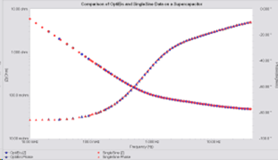
Figure 7. The comparison of OptiEIS and a single sine spectrum for a 3F ultracapacitor.

The data for the simplified Randles dummy cell is shown in Figure 8. Again the two spectra overlap perfectly. The single sine method for this measurement takes ~3hrs whereas the OptiEIS can do the same measurement within 43mins.

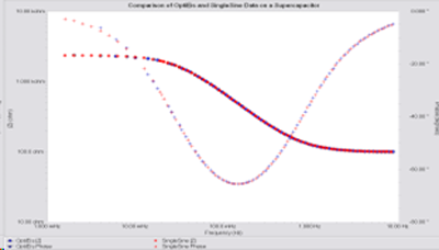
Figure 8. The comparison of OptiEIS and a single sine spectrum for a simplified Randles dummy cell (200 Ω in series with a 2.3kΩ in parallel with 2 mF).

Summary

Multiple simultaneous sine wave excitations can make EIS experiments shorter. There are a number of important issues involved with optimizing this measurement. These include system stability, linearity and simultaneous completion of the measurement at various frequencies. Good stability and linearity are achieved by keeping the overall amplitude small.

Similar completion times for all frequencies can be achieved by adjusting the applied excitation. Using the methodology described above, the experiment time can be shortened by up to a factor of about 4.

[1] Farden, D. C., Miramontes de Léon, G., and Tallman,D. “DSP-Based Instrumentation for Electrochemical Impedance Spectroscopy” Proceedings of the 195^th meeting of the Electrochemical Society, Vol. 99 No. 5, pp. 98-108, Seattle, WA (1999)

[1] “Synthesis of low-leak-factor signals and binary sequences with low autocorrelation”, IEEE Trans. On Inform. Theory, 16(1), 85, 1970

Want a PDF version of this application note?

Please complete the following form and we will email a link to your inbox!

First Name:

Surname:

Company Name:

Email address: