Square-wave Voltammetry

Introduction
Among the many electrochemical techniques available in Gamry Instruments’ Framework™ software is square-wave voltammetry (SWV), a form of pulse voltammetry. SWV is typically used in sensing electrochemically-active analytes present at low concentration. SWV, like other pulsing techniques (differential pulse, normal pulse, etc.) is more sensitive than cyclic voltammetry because the pulse current is subtracted from a baseline current to generate a differential current. SWV is unique from other pulsing techniques due to the ability to sweep across the voltage window rapidly and because of the reverse pulse. This Application Note describes what SWV is, and the parameters involved.
Quick Note on Setup
SWV is typically run on a three-electrode setup with working, reference, and counter electrodes. All three are immersed in an electrolyte and connected to a potentiostat. Cell current (Im) is measured over time between the counter and working electrodes. Cell voltage (Vf) is measured between the working and reference electrodes. SWV is a voltammetric technique so the potentiostat applies a voltage (Vsig) and measures it back as Vf while also measuring Im.
Theory Behind Square-wave Voltammetry
Voltage Waveform
We start with a staircase voltage waveform (dashed line, Fig. 1) that steps across a pre-defined voltage window. A square wave is superimposed on top of the staircase such that one square wave cycle occurs across each step (e.g. the period is equal to step duration). Summation of the staircase and square wave (solid line, Fig. 1) creates the characteristic voltage waveform used in SWV.

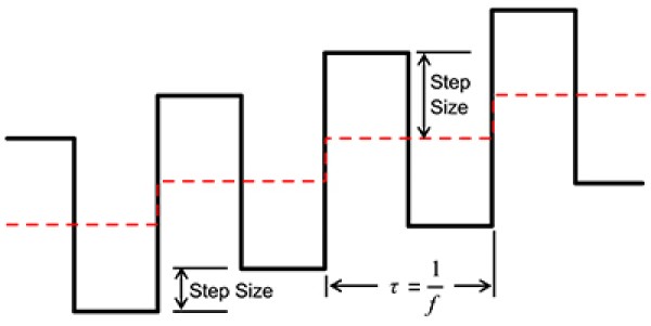
Fig. 1: Schematic of how voltage varies with time in square-wave voltammetry.
Fig. 2 shows Im and Vf over time when the characteristic waveform is applied at a Pt working electrode in the presence of a reversible redox couple. Using a reversible redox couple allows us to use Butler-Volmer kinetics to interpret Im and Vf. In this case, Vf is referenced against the open circuit potential (Eoc). When Vf is positive, Im is also positive. We expect positive Im because the applied potential is more positive than Eoc and therefore the result is a net anodic oxidation of the redox couple. Notice that halfway through the period (or step), Vf becomes negative and Im correspondingly becomes negative. Again, expected behavior since a net cathodic reduction must occur when the applied potential is more negative than Eoc. Notice that Im never reaches a steady value, which is why timing is critical. Current measured during SWV are called ‘current transients’ for this reason.
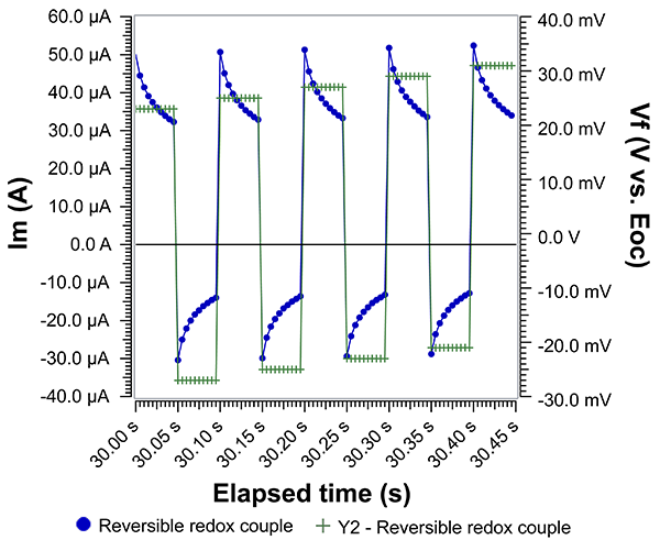
Fig. 2: Applied voltage and measured current in the presence of a reversible redox couple. Equimolar ferri-/ferrocyanide in aqueous solution with KCl as supporting electrolyte. WE: Pt disk; CE: graphite rod; RE: Pt wire pseudo-reference. Scan direction: positive.
Vfwd, Vrev, Ifwd, Irev, and Idiff
We now introduce terminology to analyze Vf and Im. Noting that the scan direction is from negative to positive potential, we assign the top of the pulse as the forward step and the bottom of the pulse as the reverse step. Therefore, in the forward pulse, Vf becomes Vfwd and Im is Ifwd. In the reverse pulse, Vf becomes Vrev and Im is Irev. Vfwd and Vrev are easily measured from Vf. However, Ifwd and Irev are not because current decays in each half-period. Thus, we must choose a time window to sample Ifwd and Irev (more on this later).
The difference between Ifwd and Irev, called Idiff, is the primary response curve of interest. Idiff is plotted against the step voltage (dashed line, Fig. 1), which is halfway between Vfwd and Vrev. Idiff is strongly dependent on how we sample Ifwd and Irev.
An actual SWV experiment does not show Im and Vf. Instead, the software automatically calculates Ifwd, Irev, and Idiff and lets you plot them against Vstep, Vrev or Vfwd.
Time, \(\tau\), for One Square-Wave Cycle and Step
Both square-wave cycle and length of a single step (dashed line, Fig. 1) in the voltage series have a duration of time \(\tau\) (s). The inverse of the cycle length is the frequency, 1/\(\tau\), or \(f\) (Hz). The duty cycle is 50%. This is the definition adopted in the Gamry Framework Software. Sometimes, in older literature, you may find \(\tau\) defined as half the square wave period, which is used out of convenience for subsequent analysis or modeling.
Scan Rate
The scan rate for a SWV experiment is inversely dependent upon the time per step, \(\tau\):
\[Scan\ rate\ (mV / s) = E\_ step/(\tau\ ) = E\_ step*f\]
The frequency used in SWV experiments typically varies from about 1 Hz to 125 Hz. Such a high f means that SWV is usually much faster than other pulsed experiments such as differential pulse.
Pulse Size
Pulse size (Epulse) sets the amplitude of the square pulse in mV. At first glance, it may seem arbitrary in scale. But in fact, pulse size should be scaled with respect to the ratio RT/nF, ~25.7 mV for a reversible, single electron transfer reaction at room temperature (n: # of electrons transferred, F: Faraday’s constant, R: gas constant, T: temperature). In the older literature, pulse size is set based on n, specifically 50 mV/n or roughly 2 * (RT/nF). See Reference #1 or #2. This is sufficient to drive the system to activate oxidation and reduction. When Pulse size is much smaller than nF/RT, then Idiff is quite small. When pulse size is much greater than nF/RT, then Idiff is controlled by diffusion (i.e. exhibits Cottrell behavior).
Optimization
Note that for a reversible electron transfer step, Estep is usually set as Estep = 10 mV/n. With initial guesses of 10 mV/n and 50 mV/n for Estep and Epulse, respectively, the frequency can be varied across a wide range of values according to log (k * f-1) where k is the rate constant of the electron transfer step (s-1). If k is unknown, then try scan rates of 10 mV/s to 1 V/s. If Estep is 10 mV, then f is 1 Hz and 100 Hz, respectively.
Lastly, the peak potential for a freely-diffusing, reversible electron transfer step should occur at: \[Epeak\ = \ E{^\circ}’ + (RT/nF)*ln\left( \frac{DR}{DO} \right)^{1/2}\]
where DR and DO are diffusion coefficients of the oxidized and reduced species and E°’ is the formal potential. Peak potential drift may be a useful indicator to interfering effects.
Parameter Setup
Below is an example of the experimental setup window from Gamry Instruments’ Framework™ software. The top half of the parameters define the voltage window in which we apply the waveform described in Fig. 1. The lower half sets certain potentiostat hardware settings. We call attention to the sampling mode in the red outlined box.

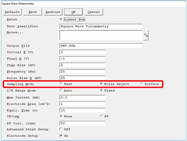
Fig. 3: Experiment setup window for square-wave voltammetry in Gamry Instruments’ Framework software. Sampling Mode (outlined in red) has three choices, Fast, Noise Reject, and Surface mode.
Cadmium in Aqueous Buffer
Fig. 4 shows a SWV example of trace detection of Cd2+ (6 ppm) dissolved in aqueous acetate buffer solution. We ran a SWV experiment at \(\tau\) = 0.1 s (i.e., frequency = 10 Hz) using a 25 mV pulse and 5 mV steps. Idiff, Ifwd, and Irev are plotted against Vstep. Note scan direction is positive voltage to negative voltage because we are detecting a cathodic reaction (e.g. Cd2+ reduction).
As Vstep approaches the E°’ of Cd2+ reduction (n=2), the absolute values of Ifwd and Irev reach a maximum. Idiff yields a single current peak. Two observations to note: 1) prior to activation, all three current values are nearly zero. 2) after activation, Idiff is nearly zero whereas Ifwd and Irev are non-zero but equal.
#1 can be explained by the fact that Cd2+ reduction does not occur at the initial voltage. And since only oxidized form is present, the reverse pulse yields zero current. The fact that all three are nearly zero indicates that the square wave is properly rejecting the contributions of any charging current (e.g. nonfaradaic current) such as from double layer charging.
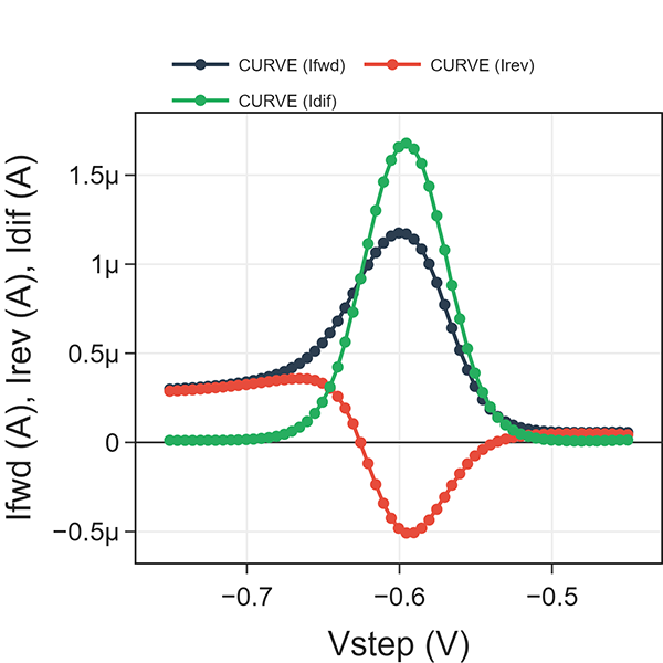
Fig. 4: Square-wave voltammetry at \(\tau\) = 0.1 s for 6 ppm Cd2+ in an aqueous acetate buffer.
#2 is explained by noting that the steady current after the peaks is the same diffusion-limited current that would flow in a sampled DC voltammetry experiment (staircase without square pulses). Here, pulses do not contribute additional current because the surface concentration of Cd2+ is zero. Thus, Idiff is also zero. In effect, SWV is able to reject the diffusion limited current that creates the familiar ‘duck’ shape in cyclic voltammetry.
Were we to vary the bulk concentration of Cd2+, the peak height would be proportional to [Cd2+]. See Reference #1. Adding another ion in solution (e.g., Pb2+) would add a second peak at a different Vstep. And because SWV rejects charging current and diffusion-limited currents, the two peaks would ideally appear side by side with minimal baseline shift. This is one of the advantages to pulse methods like SWV.
Measuring current in SWV
In this section, we discuss the importance of sampling methods in measuring the current during a SWV experiment. Simply put, we answer the question:
What is the proper way to sample current and calculate Ifwd, Irev, and Idiff?
Fast, Noise Reject, and Surface Modes
In the seminal papers describing the method of SWV, the current was sampled in a small window at the end of each pulse width (1/2 \(\tau\)). In Reference #2, they used 1/2 \(\tau\) – 7.5 µs with a sampling time of 0.04 µs, which is essentially sampling just prior to the end of the pulse. Gamry Instruments calls this method Fast mode. Such a method of sampling discriminates against any capacitive current or surface-bound reactions. The current caused by any capacitive charging or faradaic current confined to the surface decays in the initial part of the step and does not contribute to the measured current. Typically, only faradaic current caused by diffusing species is detected.
A second acquisition method is Noise Reject, which averages over the last 20% of each step. When compared to Fast mode, this improves the signal-to-noise ratio while still capturing current primarily from diffusing species. This assumes that current transient at each pulse has sufficient time to decay to a stable value such that the averaged value is similar to the Fast mode value. Fig. 5 shows that this is nominally true. But those wanting precise values should not switch between Fast and Noise Reject for replicated experiments.
With Surface mode, Gamry Instruments enables a unique sampling method to eliminate the differences between a staircase and a true ramp. In Surface mode, the current is sampled throughout the duration of a step, and is then averaged. This allows capturing both capacitive effects and any faradaic effects confined to the surface. (See our Application Note “Measuring Surface Related Currents using Digital Staircase Voltammetry.”) No other potentiostat manufacturer includes a Surface mode capability. In SWV, Surface mode samples current and averages it across each pulse (1/2 \(\tau\)).
For SWV measurements involving surface-bound reactions, we recommend using Surface mode during scanning. For everything else, such as shown in Fig. 5 and Fig 6., use Noise Reject mode. Fast mode may be preferred if wanting to replicate results from older literature. It is tempting to choose Surface mode in Fig. 5 because of the larger response. Just know that it will be more difficult to compare the experimental peak current with the estimated peak current from the well-established analytical solution for SWV.

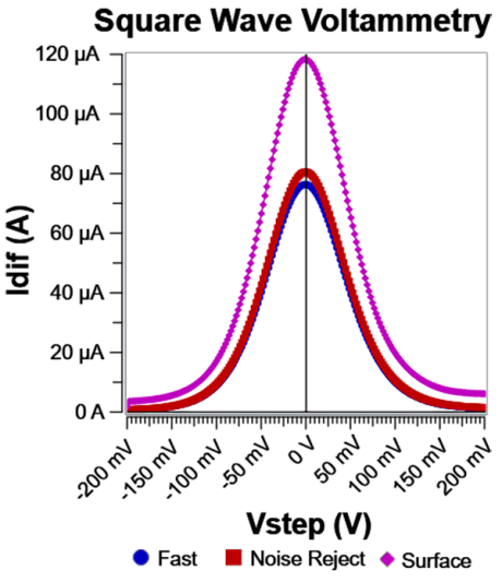
Fig. 5: Idiff for the three sampling modes. Note the baseline shift difference between Surface and Fast/Noise Reject. This is caused by double layer capacitive current being captured by Surface mode. The difference between Fast and Noise Reject is subtle, primarily around the peak current. Same system as shown in Fig. 2.

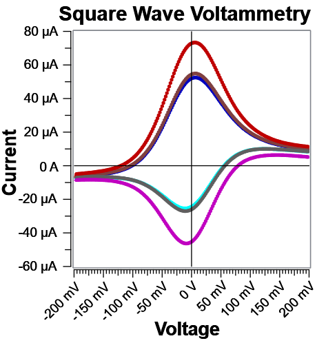
Fig. 6: Corresponding Ifwd and Irev curves for the data in Fig. 5. Notice far away from E°’, both Fast and Noise Reject discriminate against charging current effectively.
Examples
Quantitative Measurements of Trace Copper
In this example, various concentrations of copper ions in the parts-per-million range dissolved in acidified aqueous solution were scanned by SWV, along with a blank. This series of experiments (see Table 1) shows how the concentration of trace amounts of copper is directly related to the peak height.


Fig. 7: Increasing concentrations of acidified copper ions in solution, recorded with SWV.
| Scan | [Cu2+] (ppm) | Peak height @ –250 mV (µA) |
|---|---|---|
| 1 | 8.8 | 0.408 |
| 2 | 25 | 0.754 |
| 3 | 50 | 1.205 |
| 4 | 77 | 1.432 |
| 5 | 100 | 1.738 |
Comparison of Three Acquisition Modes
To show the extra sensitivity in Surface mode exclusive to Gamry Instruments’ potentiostats, Fig. 8 presents a background-subtracted set of scans using a biosensor recorded in all three modes: Fast, Noise Reject, and Surface. Clearly Surface mode is far and away the method to see the best signal for surface-bound reactions. For additional information on sampling the current transient during SWV and how to take advantage of Surface mode, see Reference #3.


Fig. 8: SWV at 100 Hz recorded in three acquisition modes on a biosensor. Blue is Fast mode, Red is Noise Reject mode, and Purple is Surface mode. All data are background-subtracted.
Surface mode verification
How do you know if Surface mode is working properly?
The best way is to test with a series RC circuit. If it helps, you may frame it as R = Ru and C = Cdl and the series RC circuit becomes a description of the impedance of a wetted electrode surface in the absence of any net faradaic reaction. (Ru: uncompensated resistance; Cdl: double layer capacitance)
Assuming a voltage scan in the positive direction, the Forward Current is the response to the "upward" voltage jump, while the Reverse Current is the response to the "downward" jump back. The forward jump and reverse jump are drawn out schematically in Fig. 9.
To understand the current responses, first calculate the total voltage jump that drives them, using Epulse and Estep:
Forward Jump: To reach the new peak, the voltage must recover from the bottom of the previous cycle and climb the new staircase step. \[Vfwd\ = \ 2\ *\ Epulse\ + \ Estep\]
Reverse Jump: The voltage simply drops from the peak to the trough of the current cycle. \[Vrev\ = \ - 2\ *\ Epulse\]
Because the Forward jump includes the step height, it is fundamentally larger than the reverse jump. In Surface mode, the Forward Current will therefore be slightly larger than the Reverse Current, and the "leftover" current after they cancel out is proportional to the Step Height. Note that the reverse current will be negative as the step direction is reversed.

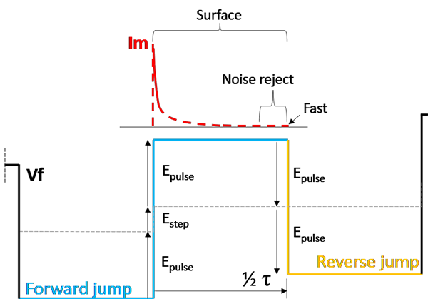
Fig. 9: Schematic for estimating surface-bound currents using Surface mode in SWV.
When integrating the current across the entire step, the resistor determines how fast the charge moves, but the capacitor determines how much total charge is stored. Assuming the step duration (1/2 \(\tau\)) is long enough for the capacitor to fully charge (longer than 5x the RC time constant), the total charge is simply the capacitance multiplied by the voltage change. The average current is then this total charge divided by the step duration. \[Ifwd\_ avg\ = \ C\ *\ (2\ *\ Epulse\ + \ Estep))\ /\ (1/2\ \tau)\] \[Irev\_ avg\ = \ (C\ *\ 2\ *\ Epulse)\ /\ (1/2\ \tau)\]
It is important to note here that timing is critical, just as we discussed earlier. 5x the RC time constant is a good guide for setting the frequency of the SWV experiment. In the case of a real sample, the time constant that sets the upper frequency limit is Ru*Cdl (f = 1/(Ru*Cdl)). Setting frequencies higher than this will not yield any meaningful results. In a typical 3mm disk electrode experiment, Ru and Cdl might be 10 ohm and 100 µF, respectively. The time constant is 1 ms and frequency is 1000 Hz. Divide that by five to get 200 Hz and this would be a good guide to the upper frequency of a SWV experiment.
Sample Data
Let’s set R = 200 Ω and C = 1µF. Apply a square wave with the following parameters: \[Scan\ range:\ 0V\ - \ 1V\] \[Estep:\ 2\ mV\] \[Epulse:\ 50\ mV\] \[Frequency:\ 25\ Hz\ (\tau:\ 0.04\ s)\]
From these parameters, forward current and reverse current in Surface mode are: \[Ifwd\_ avg\ = \ 1\ µF*(2*0.052\ V)\ /\ 0.02\ s\ = \ + 5.2\ µA\] \[Irev\_ avg\ = \ 1\ µF*(2\ * - 0.05\ V)\ /\ 0.02\ s\ = \ - \ 5.0\ µA\]
Fig. 10 shows experimental data on our series RC circuit. The average value for Ifwd is 5.16 µA ± 5 nA and Irev is -4.93 µA ± 5 nA, which is exactly what we expected. And as a sanity check, enabling Fast mode resulted in Ifwd and Irev average values of ~91 nA, which is simply the offset current on the 1 mA I/E range. Lastly, we check timing by noting that five times the RC time constant, 1 ms, is smaller than our step duration, 20 ms. Therefore, we know that the capacitive response is fully captured during the step when Surface mode is active.

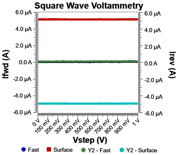
Fig. 10: Sample data run on a series RC circuit with Surface mode and Fast mode. Surface mode captures all of the capacitive charge and calculates an average current.
Setting current range
Note that although the currents are quite low, the max current is determined at time zero in the step by Ohm’s Law: \[Ifwd,max\ = \ Vfwd\ /\ R\ = \ 0.104\ V\ /\ 200\ \mathrm{\Omega}\ = \ 52\ µA\]
Thus, to integrate properly in Surface mode, the I/E range should be set according to max current in the step. In this case, 100 µA range or 1 mA range would do. We chose the latter for this experiment. The accuracy for this current range is within ±500 nA (max value). Voltage noise is expected to induce background currents of ~5 nA. As such, it is not surprising to see nA-level error in this analysis.
Finally, RC components were checked by impedance method (EIS): \[R\ = \ 0.999 \pm 0.003\ µF\] \[C\ = \ 199.8 \pm 0.8\ \mathrm{\Omega}\]
Further reading
Reference #1: Anal. Chem. 1977, 49, 13, 1904–1908
https://doi.org/10.1021/ac50021a009
Reference #2: J. Phys. Chem. 1983, 87, 20, 3911–3918
https://doi.org/10.1021/j100243a025
Reference #3: Anal. Chem. 2024, 96, 23, 9561–9569
https://doi.org/10.1021/acs.analchem.4c01053
Conclusion
Square-wave voltammetry is a rapid means of qualitatively and quantitatively determining analyte even at low concentrations in a solution. Optimization of the SWV parameters requires an understanding of the timing of your electrochemical response and setting an appropriate frequency or \(\tau\). The older literature frames SWV parameters in terms of reversible reactions involving diffusing species. However, this guidance is often not optimal for surface-bound reactions.
That’s why we offer Surface mode, which allows you to sample the entire current transient in SWV. By turning Surface mode on and off, you can estimate the surface-bound contributions to the current transient earlier in the pulse time. We recommend users start by determining the timing of the electrode response by using EIS. Estimate Ru and Cdl to calculate the RC time constant and use this as the upper guide for the frequency and subsequent SWV parameter optimization.
Found this appnote helpful? Let us know on LinkedIn!
https://www.linkedin.com/company/gamry-instruments
Application Note Square-wave Voltammetry Rev. 1.0. 1/26/2026. \(©\) Copyright 2026 Gamry Instruments, Inc. Interface, Reference, and Framework are trademarks of Gamry Instruments, Inc.
Want a PDF version of this application note?
Please complete the following form and we will email a link to your inbox!
Categories