Pulsed Electrochemical Deposition

Tracking electrodeposition with redox replacement using an electrochemical quartz crystal microbalance

Daniel Molina Montes de Oca^a,* and Jerome T. Babauta^b

^a Idaho National Laboratory; Idaho Falls ID, USA

^b Gamry Instruments; Warminster PA, USA

* Corresponding author:

daniel.molinamontesdeoca@inl.gov

Introduction

In this application note, we introduce the reader to a pulsed electrochemical deposition technique and how electrochemical quartz crystal microbalance (EQCM) can provide additional insight into the processes that occur during each of its cycles. Electrodeposition with redox replacement (EDRR) is a technique that can enable the recovery of precious metals like Ag, Au, and Pd, present at trace levels in process streams that contain a high concentration of less noble metals such as copper. Because of the low concentration of the precious metal, traditional electrowinning would include an unacceptable level of co-deposition of the non-noble metal. Instead of continuous deposition, EDRR uses repeating short electrodeposition pulses followed by longer open circuit periods. Due to the difference in reduction potentials, during the open circuit periods, the trace precious metal in solution spontaneously replaces the less noble metal that was electrodeposited.¹ The EQCM can be used to study EDRR and track electric potential, current, and mass transients involved in each EDRR cycle.² This application note highlights results from EDRR on an EQCM flow cell, from a sulfuric acid solution that contains silver and copper ions.

Reactions and pulse waveform

Cu and Ag are electrodeposited simultaneously during the constant potential electrodeposition (ED) section of the EDRR cycle according to Eq. 1 and Eq. 2 below. In our case, Ag is the metal of interest and Cu is the interfering metal.

(1) (2)

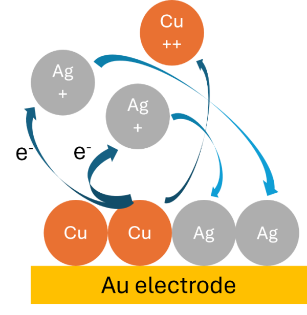
Once the mixed Cu and Ag metal film is formed, the applied potential is interrupted, and the system is left open (cell switch open). The expected reaction during this open circuit section of the EDRR cycle is shown in Eq. 3. (3)

This is a spontaneous reaction, with a positive reduction potential change of 0.46 V under standard conditions. The net effect of Eq. 3 is a replacement of Cu atoms with Ag atoms in the film. Hence the name ‘redox replacement’. Figure 1 shows a possible mechanism of how the spontaneous reaction might occur. Given enough time, all available Cu(s) is replaced by Ag(s). Since all this occurs at open circuit, the measure of how far the EDDR has proceeded is the open circuit potential (OCP).

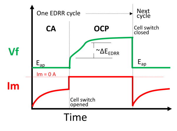
The entire EDRR cycle is schematically drawn out in Figure 2. The first half of the cycle is a constant voltage, chronoamperometry (CA) step where an appropriate voltage is applied to activate Eq. 1. Redox replacement proceeds in the second half of the cycle when CA is stopped to measure the OCP. During the OCP step, the voltage increases as Cu(s) is replaced by Ag(s) and this is referred to as .

Experimental Setup

An 8 MHz Au EQCM electrode was housed in a 50 μL flow cell, with RE and CE electrodes housed in a separate anolyte compartment ionically connected by a ceramic frit. A 0.5 mL sample containing 5 mM CuSO₄ and 0.5 mM AgNO₃ was pumped through the cell at 0.2 mL/min using a 0.5 M H₂SO₄ carrier solution, while EDRR cycles were applied with a deposition time of 0.2 s (at E_ap = -0.1 V_ag/AgCl) and a redox replacement time of 10 s. The experimental setup is described in more detail by Molina et al.²

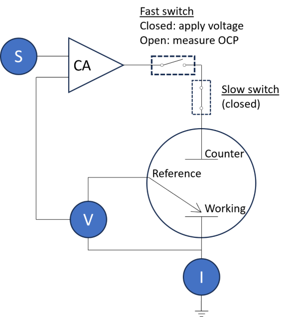
The flow cell was connected to an eQCM10M™ Quartz Crystal Microbalance¹ which was coupled to an Interface™ 1010E potentiostat. Both instruments were connected to a single computer with Gamry Software installed. The Resonator™ software was used to collect QCM data (i.e. frequency shift). The Framework™ software was used to run a custom chronoamperometry script designed for rapid, intermittent application of a constant voltage in between periods of OCP. Note that this is distinct from typical voltage pulsing and is required in this scenario because the voltage must be allowed to float during the redox replacement step.

Figure 3 shows the simplified schematic. In this case, the potentiostat continuously applies the signal, S, which is a constant voltage, . When the “fast switch” is closed, the working electrode potential is set at , and current is allowed to flow. When the “fast switch” is open, no current flows through the working electrode and thus the OCP is measured. During this time, the “slow switch” is always on. This method of control allows fast switching at the μs-scale! Thus the 0.2s pulse used here was very easily applied and ample data points were measured. Why is timing and speed so important? It is because the instrumentation should be able to electrodeposit fine amounts of material to determine sensitivity of EDRR. 0.2s pulse was optimal for the flow cell geometry used here, but perhaps shorter pulses may be required for other geometries. In other words, the setup and scripts used here can accommodate a wide range of operating conditions so long as the user has an eQCM setup from Gamry.

Results and discussion

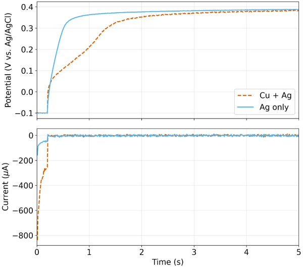
Figure 4 shows the potential (top panel) and current (bottom panel) during EDRR after the Ag/Cu sample is injected into the H₂SO₄ carrier stream and allowed to permeate the flow cell. For purposes of comparison, the potential and current response for sample injection with Ag only under identical conditions is also shown (blue solid trace). During the 0.2s polarization pulse, cathodic current is measured as both Cu and Ag co-deposit, with the majority being Cu. Once the “fast switch” (see Figure 2 and Figure 3) was opened, the potential increased rapidly for both the Ag/Cu sample and the Ag only sample. The Ag only potential smoothly transitioned to a stable OCP of 0.398 V_Ag/AgCl, which was very close to the theoretical equilibrium potential of 0.407 V_Ag/AgCl, calculated using the Nernst equation and a bulk concentration of 0.5 mM of Ag⁺. The Cu + Ag potential increased quickly to ~0.05 V_Ag/AgCl, which was consistent with the theoretical equilibrium potential of 0.075 V_Ag/AgCl, again calculated using the Nernst equation and a bulk concentration of 5 mM Cu⁺². However, the potential was not stable due to redox replacement (see Eq. 3). The initial Cu film transitioned to a purely Ag film and the potential response reflected this as the final potential at five seconds was nearly identical to the Ag only case. Note that during the entire window of redox replacement, current was exactly zero as there was no physical path for electrons to flow.

The EQCM frequency shift () during the same experiment is shown in Figure 4 alongside the potential and current. Three distinct zones can be observed: (1) a sudden mass increase² due to electrodeposition during the first 0.2 s of the cycle (2) a zone with a net mass increase due to redox replacement (3) a zone of practically no mass change indicating either very slow or no redox replacement. In zone two, there is a net mass change because two heavier silver atoms replace one copper atom, but there are other processes (Cu corrosion for instance) that can cause Cu to leave the surface during the same period. Since there is a net mass change according to the EQCM signal, we can conclude that this opposing effect is smaller compared to the mass gain through redox replacement.

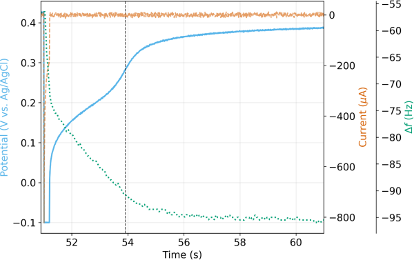
Digging deeper into the data, we estimate a total charge of 61.5 μC was injected during electrodeposition. As a first approximation, let us assume 100% of the charge resulted in Cu(s) formation. Thus, by Faraday’s law of electrolysis, this is equivalent to 20.2 ng of copper plating onto the QCM sensor. Based off the verified calibration factor of 0.57 Hz/ng ², this should result in a net frequency shift of -11.5 Hz. Looking at Figure 4, we observe an experimental frequency shift of -16.4 Hz. The fact that the experimental value is larger indicates our initial assumption of 100% Cu(s) is incorrect. This further indicates that the initial charge injection of 61.5 μC includes a contribution from Ag(s) formation. By setting up a simple system of equations, one can back calculate the percentage of the initial charge due to Ag(s) formation. One equation is a balance around total charge. A second equation is a balance around the total frequency shift observed (i.e. a mass balance). With two equations and two unknowns, the percentage is readily calculated as 17.6%. Meaning, 10.8 μC (12.1 ng of Ag(s)) of initial charge came from Ag(s) formation and 50.7 μC (16.7 ng of Cu(s)) from Cu(s) formation. The total mass of 28.8 ng resulting in the total -16.4 Hz frequency shift observed during electrodeposition. In this case, the atomic ratio Cu:Ag is 2.35 in the deposit right after the pulse, which is lower than the 10:1 ratio in solution, suggesting there’s already an enrichment of Ag, possibly due to faster deposition for Ag caused by a larger exchange current density and overpotential governed by Butler-Volmer kinetics.

Let us now assume the redox replacement goes to completion and all of the Cu(s) is replaced by Ag (s). From (3), we know the 1:2 Cu:Ag stoichiometry. The resulting mass of Ag(s) is calculated to be 56.6 ng, assuming all moles of Cu(s) are replaced. The net mass gained is then 56.6ng minus the initial 16.7 ng of Cu(s), or 39.9 ng. Again, using the verified calibration factor of the crystal², the expected frequency shift induced by this net mass gained is 22.8 Hz. Looking at Figure 4, the experimental frequency shift from immediately after the pulse to the end of the OCP step is 22.9 Hz, nearly identical to the calculated value! Thus, we prove through EQCM that the potential response we discussed in Figure 4 tracks the gradual but complete redox replacement of Cu(s) by Ag(s).

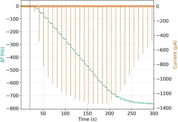
Of interest is the inflection point in the voltage (vertical dashed line in Figure 4) that likely represents some kind of transition from a kinetically-constrained regime to one where mass transfer limits the replacement rate. This could be interpreted as Ag passivating over Cu domains. Given that the molar volume of Ag(s) is ~15% larger than Cu(s)and the fact that two Ag atoms replace one Cu atom, such an interpretation seems plausible. However, corroboration of such phenomena requires additional supplementary evidence. Lastly, Figure 5 provides a zoomed-out view of the entire series of pulses as the sample volume travels through the system. Multiple cycles of EDRR can be applied sequentially without issue and Ag(s) can be concentrated onto the sensor surface.

Conclusions

Here we show how EQCM can be used to track the spontaneous redox replacement of Cu(s) by Ag⁺¹ ions. When done correctly using a stable and well-designed flow cell setup, a very accurate accounting of charge and mass can be made. For additional details, we refer readers to the original article that shows how simple variation of operating conditions, such as the redox replacement time, can produce very different results in the observed frequency and potential signals during EDRR².

Ultimately, this application note gives readers a clear example of how EQCM can track coupled chemical reactions that do not result in a net current or net charge at the electrode surface. In the case of EDRR, we just so happen to know that the OCP could also be used to track EDRR. But one could imagine replacement reaction mechanisms that do not induce an OCP change or where the OCP itself is poorly defined. In these cases, EQCM could still track the transformation of the electrodeposited film.

References

1. P.-M. Hannula, S. Pletincx, D. Janas, K. Yliniemi, A. Hubin, and M. Lundström, Surface and Coatings Technology, 374 305-316 (2019). https://doi.org/10.1016/j.surfcoat.2019.05.085

2. D. E. Molina, N. Wall, H. Beyenal, and C. F. Ivory, Journal of The Electrochemical Society, 168 (5), 056518 (2021). https://doi.org/10.1149/1945-7111/abfcdd

Found this appnote helpful? Let us know on LinkedIn!

https://www.linkedin.com/company/gamry-instruments

Application Note Tracking electrodeposition with redox replacement using an electrochemical quartz crystal microbalance Rev. 1.0. 3/31/2026. Copyright 2026 Gamry Instruments, Inc. Interface, Resonator, and Framework are trademarks of Gamry Instruments, Inc.

---

1. The eQCM 15M™ is the successor to the original eQCM 10M™. See: https://www.gamry.com/quartz-crystal-microbalance/eqcm15/↩︎

2. According to the Sauerbrey equation, mass and frequency shift have a negative correlation where a positive mass increase results in a negative frequency shift. See: https://www.gamry.com/application-notes/qcm/basics-of-a-quartz-crystal-microbalance/↩︎

Want a PDF version of this application note?

Please complete the following form and we will email a link to your inbox!