Low impedance batteries and the Interface 5000E Potentiostat/Galvanostat
In this technical note, we take a look at low impedance batteries and how the Interface 5000E (IFC5000) performs when running EIS. First, let us define what we mean by “low impedance” for single cells. Battery material testing in coin cells typically shows impedances in ohms. Cylindrical cells in the single digit A*hr range exhibit impedance in the tens of mΩs. Larger form factor batteries like pouch cells exhibit impedance less than a mΩ. Of course, this is sort of a rule-of-thumb for Li-ion based batteries, but it’s useful to relate to. The discharge rate—how much current the battery can provide—is more indicative of its impedance instead of the form factor. Thus, this technical note is really about high discharge rate batteries that show low impedance response. Here we define a low impedance as any single battery cell that measures <1 mΩ at least once within a measurable frequency range and call special attention to them for two practical reasons:In this technical note, we take a look at low impedance batteries and how the Interface 5000E (IFC5000) performs when running EIS. First, let us define what we mean by “low impedance” for single cells. Battery material testing in coin cells typically shows impedances in ohms. Cylindrical cells in the single digit A*hr range exhibit impedance in the tens of mΩs. Larger form factor batteries like pouch cells exhibit impedance less than a mΩ. Of course, this is sort of a rule-of-thumb for Li-ion based batteries, but it’s useful to relate to. The discharge rate—how much current the battery can provide—is more indicative of its impedance instead of the form factor. Thus, this technical note is really about high discharge rate batteries that show low impedance response. Here we define a low impedance as any single battery cell that measures <1 mΩ at least once within a measurable frequency range and call special attention to them for two practical reasons:
- The battery impedance is on the same order of magnitude or lower than the contact resistance measured using the standard alligator clips included with most commercial potentiostats. Users must make custom connections to low impedance batteries.
- Instrumentation: Not all potentiostats (really galvanostats) can make these measurements. Usually, potentiostat hardware design decisions trade EIS accuracy for reduced manufacturing cost at the extreme. This is where the specifications look good on paper but fail when put to the test.
How can you tell if your potentiostat can make low impedance measurements?
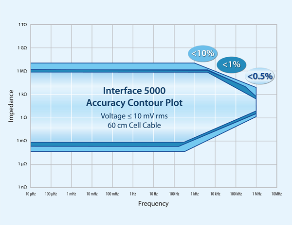
Figure 1. Accuracy contour plot of the Interface 5000E potentiostat with emphasis in the low impedance range.
First take a look at the accuracy contour plot (ACP). Figure 1 shows the ACP for the IFC5000. You can see accuracy falls off as you go below the 1 mΩ threshold. That means you must be skeptical of any impedance data measured below 1 mΩ. For a Gamry potentiostat, you can nominally estimate the lowest measurable impedance as Z_low (I_max)=1mV/(2×I_max ). I_max is maximum current at the highest current range. 1 mV is a simple guideline we use for the AC voltage response during galvanostatic EIS. You can technically measure much smaller, but we won’t cover that topic here. The factor of two accounts for the ±5A, or peak-to-peak span of the AC signal. For the IFC5000, Z_low evaluates to 100 µΩ. There is also an upper frequency limit determined by the cable inductance. Our standard 60 cm cell cable nominally exhibits <100 nH of cable inductance. Remember, longer cables exhibit larger cable inductance! You can use the cutoff frequency (f_c) for a simple RL circuit to estimate the upper frequency limit where f_c (R,L)=R/2πL (Hz). Thus f_c (1mΩ,100nH) would be evaluated to be about 1600 Hz. Realistically, expect to use ≤1 kHz as the upper frequency limit in EIS for low impedance systems because you typically need to add extra cabling to reach your battery on the bench, in a rack, or in some kind of environmental chamber. See this application note on cabling for additional information: https://www.gamry.com/application-notes/EIS/accurate-eis/.
Testing the limits
You must check the accuracy of your potentiostat after estimating its capability using an ACP. The easiest way to do so is to buy a robust current shunt rated to pass I_max current. For this testing, we obtained a 100 µΩ current shunt that is rated to measure 50 mV when 250A is applied. Note that a proper current shunt will have a four-terminal layout where the outer two terminals carry the current. The inner two terminals are used to measure the voltage drop—details on measurement of shunts can be found within the application note https://www.gamry.com/application-notes/EIS/low-impedance-limits-with-the-gamry-reference-30k-booster/. Figure 2 shows the impedance spectrum as a Bode plot recorded during a galvanostatic EIS test on the shunt. As expected, the high frequency impedance is controlled by the cable inductance where phase angle is positive and Zmod is decreasing as the frequency decreases. At 1kHz (vertical red dashed line), you can see a mixed response and below 10 Hz the impedance is fully resistive (blue arrow) i.e. the phase angle reaches 0°±1°. The inset shows the series RL model that was used to extract R_shunt and L_stray from the data, which were 100 µΩ ± 0.30µΩ and 10.7nH ± 0.05nH, respectively. Using these fit values f_c evaluates to 1487 Hz, which is consistent since the measured phase angle in Figure 2 is 45° at that frequency. The results show that the IFC5000 is capable of measuring impedances as low as 100 µΩ. In fact, it can measure even lower with diminishing accuracy.
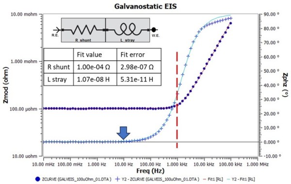
Figure 2. Impedance spectrum from a galvanostatic EIS test on a 100 µΩ current shunt. Iac was 3.5Arms (4.95Apk) and Idc was 0A
Low impedance battery results and modeling
Let’s take a look at the impedance response of a commercial lithium iron phosphate battery with a 302 Ah (~1 kWh) battery capacity as shown in Figure 3. The inset table lists battery specs pulled from the data sheet. Just like the shunt EIS experiment above, this EIS spectrum was collected with Iac of 3.5Arms (4.95Apk) and Idc of 0A. The impedance results show an estimated HFR of ~206 µΩ (@125 Hz), which is consistent with the nominal resistance tolerance. However, a better estimate is obtained by fitting the impedance data to an equivalent circuit.
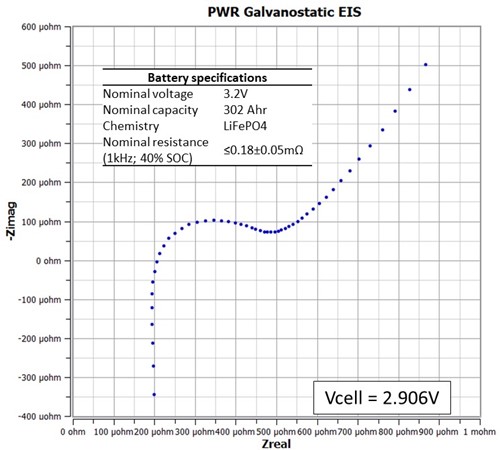
Figure 3. Nyquist plot showing the LiFePO4 battery impedance response at a cell voltage of 2.906V. The cell was discharged at 0.2C until a voltage cutoff of 2.8V. It was left overnight, and impedance was measured the following morning.
Because we know little about the battery internals, we have chosen an equivalent circuit that has the minimum number of fit parameters that gives operational parameters of HFR, L_stray, R_int, C_int, and CPE_lowfreq. They describe this impedance spectrum only and may be unsuitable for the battery impedance measured under another condition (i.e. higher SOC value). Those familiar with EIS EEC modeling may recognize this EEC as a simple Randle’s cell with generalized CPE modeling the low frequency “tail”. The fact that this EEC works implies that the anode and cathode impedance responses are indistinguishable under the test condition. Figure 4 shows the EEC model results on top of the impedance data. While the overall fit trend is correct, frequencies with a poor fit are noticeable and is expected since we used a capacitor element to model high frequency capacitance. This just means the high frequency capacitance is non ideal, and using a CPE could help improve the fit, which is shown in Figure 5. Table 1 compares the EEC parameter values for both model fit results. Below is a discussion by each EEC element. One thing to note is that all parameter errors are smaller than the corresponding parameter values. This is an important check to ensure you are not overparameterizing the analysis.
Lstray
Stray inductance is estimated at ~70 nH and is minimally affected by the choice of capacitor element (C vs CPE). Less than 100 nH is typical.
HFR
High frequency resistance is a critical parameter for many. We estimated three values for HFR depending on the method: 1) 206 µΩ (graphically via Nyquist plot) 2) 198 µΩ (EEC analysis w/ C_int) and 3) 182 µΩ (EEC analysis w/ CPE_cap). We would expect the third estimate to be the most accurate of the three.
R_int
This lumped resistance is the sum of all contributions in the device such as charge transfer and transport. It has too many dependencies that a single impedance spectrum analysis cannot adequately analyze it.
C_int / CPE_cap
This lumped capacitance is typically associated with double layer capacitance in simple electrochemical systems (wetting of a flat electrode surface by the electrolyte). However, in batteries that have many interfaces, it is difficult to say what fraction of this observed capacitance is contributed by true double layer behavior.
|
CPE_lowfreq
This element is the most ambiguous in this EEC. In series with R_int, this element accounts for all non-resistive behavior in the charge transfer branch. It is observed at lower frequencies than C_int/CPE_cap, which is why we refer to it as “lowfreq”. Two sources of low frequency non-resistive behavior are transport phenomena (i.e. Warburg-type impedances) and buried interfaces (i.e. porous electrode behavior). Pseudo-capacitance from plating/stripping can also show up here.
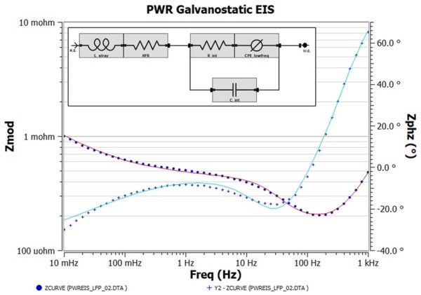
Figure 4. Bode plot corresponding to Figure 3 with the EEC (inset) fit overlay on top. Fit results are shown in Table 1.
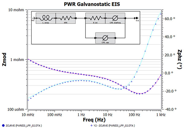
Figure 5. Bode plot corresponding to Figure 3 with the EEC (inset) fit overlay on top. The capacitor in Figure 4 is replaced with a CPE to account for non-ideal capacitive behavior. Fit results are shown in Table 1
Table 1. Parameter values based on the EEC fit results for the battery. CPEs have two parameters, Yo and α, following this equation, Z_cpe=1/(Yo(jω)^α ). Yo is the CPE coefficient and α is the exponential factor. Yo has units of s^α/Ω while α is unitless.
|
EEC parameter |
Figure 4 |
Figure 5 |
|||
|
Value |
±Error |
Value |
±Error |
||
|
L_stray |
70.29 nH |
1.13 nH |
73.04 nH |
1.35 nH |
|
|
HFR |
197.83 µΩ |
2.23 µΩ |
182.55 µΩ |
4.28 µΩ |
|
|
R_int |
229.74 µΩ |
5.74 µΩ |
295.97 µΩ |
1.29 µΩ |
|
|
C_int |
27.64 |
1.00 |
--- |
--- |
|
|
CPE_cap |
Yo |
--- |
--- |
70.91 |
10.49 |
|
α |
--- |
--- |
0.81 |
0.03 |
|
|
CPE_lowfreq |
Yo |
5381.52 |
193.31 |
6785.92 |
374.60 |
|
α |
0.46 |
0.01 |
0.53 |
0.02 |
|
|
Goodness of fit |
11.23e-04 |
--- |
3.02e-04 |
--- |
|
Alternative EEC models
So far, we have not mentioned anything about specific battery processes. For example, we have not discussed the solid-electrolyte interphase (SEI) layer or the cathode-electrolyte interphase (CEI) layer and how that would show up in the data. We haven’t even touched on the topics of anode or cathode impedance responses. We could have formulated an EEC similar to what we suggested in our other application note (Figure 9, https://www.gamry.com/application-notes/battery-research/testing-lithium-ion-batteries/). Figure 6 shows how we can simplify the series configuration based on the observation that there is only a single time constant in the Nyquist curve. Results of the assumption and fitting routine are shown in Table 2. Comparing Table 2 to Table 1 shows that both models yield similar results. Unfortunately, this is one of the major limitations of the EEC method. This is why it is critical to measure battery impedance data across multiple battery conditions.
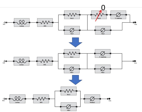
Figure 6. An example of a series EEC configuration and how to simplify based on the assumption that one of the Rct elements is not observed in the impedance data.
Table 2. Fit results for the EEC in Figure 6.
|
EEC parameter |
Figure 6 EEC (series configuration) |
||
|
Value |
±Error |
||
|
L_stray |
73.32 nH |
1.34 nH |
|
|
HFR |
180.3 µΩ |
4.14 µΩ |
|
|
R_ct,1 |
289.1 µΩ |
12.43 µΩ |
|
|
CPE_dl,1 |
Yo,1 |
81.43 |
10.77 |
|
α,1 |
0.80 |
0.03 |
|
|
CPE_total |
Yo,total |
6699 |
393 |
|
α,total |
0.53 |
0.02 |
|
|
Goodness of fit |
2.24e-04 |
--- |
|
Conclusion
This technical note addresses EIS measurements with low impedance (less than 1 mΩ) lithium-ion batteries. We recommended first testing the potentiostat capability to measure low impedance. We show how that can be accomplished with a current shunt. Afterwards we discuss battery impedance measurements by using a simple equivalent circuit model.
Want a PDF version of this application note?
Please complete the following form and we will email a link to your inbox!
Categories